You can make negative numbers red in Google Sheets easily. I have shared three different ways to make any type of – negative number in Red color or even in any other different color.
Negative numbers are those that are less than zero, and Excel automatically prefixes them with a minus symbol. If you use Google Sheets to keep tabs on your finances, you’re bound to come across some negative statistics. To make negative numbers more visible, you can have them show in red automatically, which is considerably more visible than a minus sign or parenthesis.
The three approaches to make negative numbers red in Google sheets are:
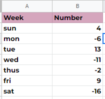
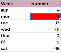
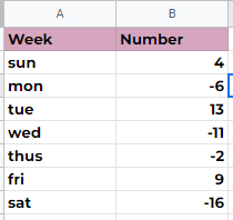
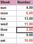
Assume you have the following dataset.
Read more: How to Make a Gantt Chart in Google Sheets
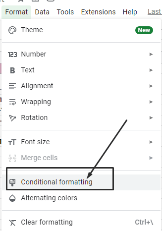
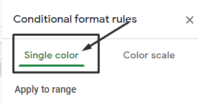
You can format a cell based on its contents using conditional formatting. With conditional formatting, it is possible to change the font color of negative numbers without changing the format.
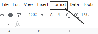
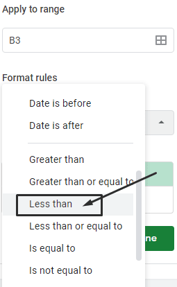
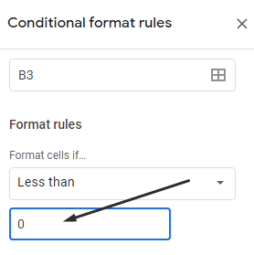
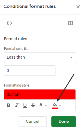
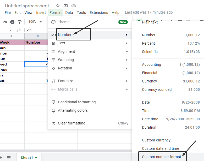
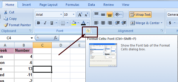
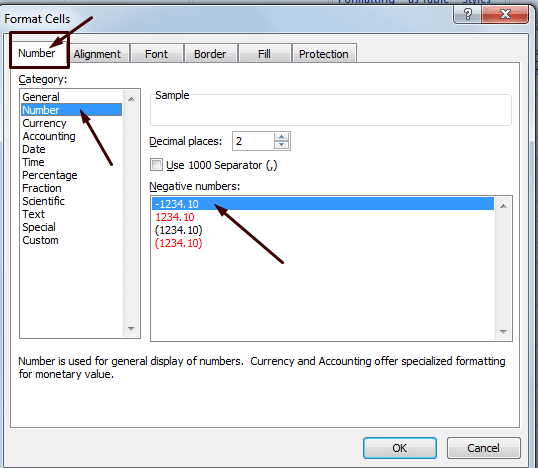
To make negative numbers red in Google Sheets, follow these simple steps:
Read more: How to Create a Graph in Google Sheets
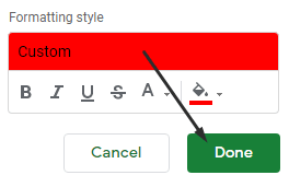
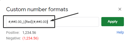
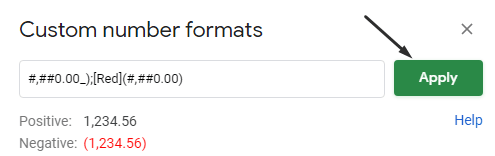
Using a custom number format in Google Sheets, you can turn a range of cells red. This will highlight only negative numbers.
Now, despite everything else in your dataset remaining the same, the negative numbers would be highlighted in red.
Read more: How to Make a Spreadsheet in Google Docs
You can also choose from many number formats if you use custom number formatting:
Read more: How to Group Worksheets in Excel
Read more: How to Make a Timeline on Google Docs
Conditional Formatting should be used with caution when displaying negative numbers since it reassesses its condition and applies to format again if the number changes. You can even change the colour of the text using custom formatting. However, Text formatting does not support colours.
A variety of colors are available, including black, red, blue, yellow, and green. So, I’ve listed 3 ways to make cell values with negative values stand out in red. I prefer to format negative numbers using custom formatting instead of using built-in functions in most programs.
This post was last modified on February 9, 2022 00:07
Learn how to increase virtual memory in Windows 11, which in turn will improve system…
Learn how to remove OneDrive from File Explorer in Windows 11 with account unlinking, Group…
Learn how to find largest files on Windows 11 with File Explorer, Storage Settings, and…
Learn how to turn off OneDrive on Windows 11 by going to sync settings, unlinking…
Learn how to insert calendar in PowerPoint with templates, tables, or Excel. Present professional and…
Learn how to create templates in Outlook, which in turn will save you time, improve…
This website uses cookies.