I have shared three ways to truncate text in Excel. You can use this method in 2013, 2016 and 2019 Excel. You can truncate any type of text or number.
Excel reports contain two components. Both the text and the numerical components. Moreover, If the text makes up a significant portion of the data contained in your spreadsheet, you might need to make some adjustments to ensure that everything fits correctly. Due to the fact that TRUNC works only with numbers in Microsoft Excel, this is the procedure you must follow.
We need to automate reporting because doing so reduces the amount of effort and time required, as well as improves accuracy. We can work with Text in Excel using many functions, but there are still some situations that require creative use of the existing tools.
Read more: How to Cross Reference Two Lists in Excel
How to Truncate Text in Excel
By truncating text in Excel, we mean slicing it at multiple spots to reduce its length to our requirements. With the Excel TRUNC function, you can return a truncated number that is based on the original number and the number of digits in it. Its objective is to reduce a number to a specific decimal point. The syntax for it looks like this: =TRUNC (number, [num digits]).
Read more: How to Create Slicers in Excel
How to truncate text in excel based on character?
Sometimes a list of strings has some lengthy characters, and you may like to trim them for organizational purposes. Moreover, Excel’s text-editing features are numerous and effective. A cell can be truncated by using three of these functions:
- RIGHT
- LEFT
- MID
Read more: How To Calculate Square Root in Microsoft Excel
Method 1. RIGHT
A single-byte character set (SBCS) can be counted by using the RIGHT function, while a double-byte letter set (DBCS) can be counted by using the RIGHTB feature (DBCS). With the exception of this one distinction, these functions do exactly the same actions. Therefore, you are free to employ whichever method works best for you to truncate text in Excel.
First, each formula has two syntaxes: RIGHT(text, number of characters) and RIGHTB(text, number of bytes). You can input the cell value and maintain the contents of the right-hand pane.
- Open the Excel spreadsheet application.
- Choose the cell where the truncate text in Excel will display.
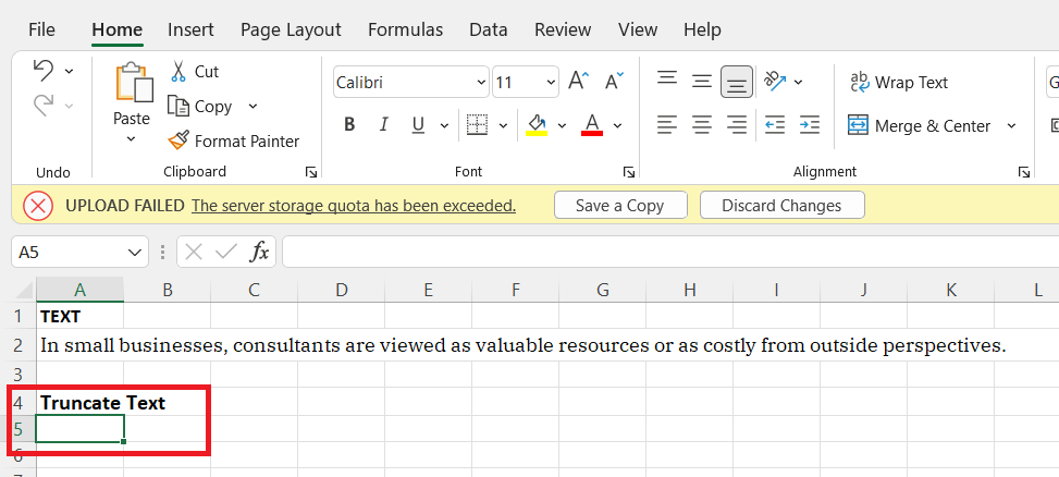
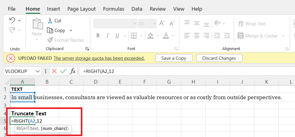
- Enter the RIGHT formula in the cell you’ve chosen.i.e: =RIGHT(A2,12)
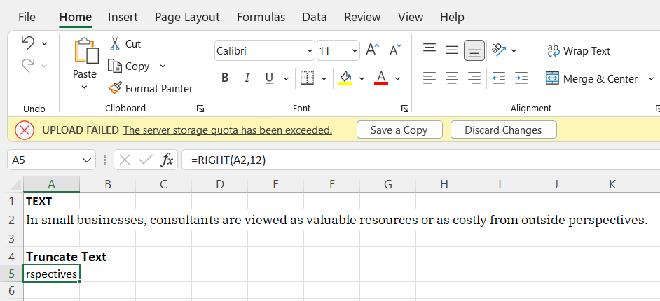
- Click Enter once the formula is complete.
Read more: How to Add a Secondary Axis in Excel
Method 2. LEFT
In terms of the LEFT and LEFTB methods, they’re similar to the RIGHT and RIGHTB methods, and you can either use characters or bytes. However, these functions allow you to shorten your text string in the opposite direction.
Both LEFT(text, number characters) and LEFTB(text, number bytes) require that the cell reference be inserted with the first argument in each formula.
- All two steps are exactly the same as described above.
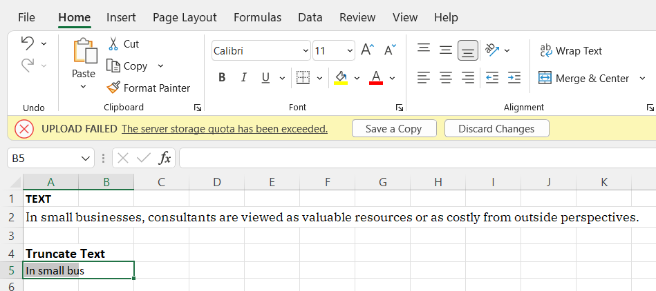
- Enter the LEFT formula in the cell you’ve chosen.i.e: =LEFT(A2,12)
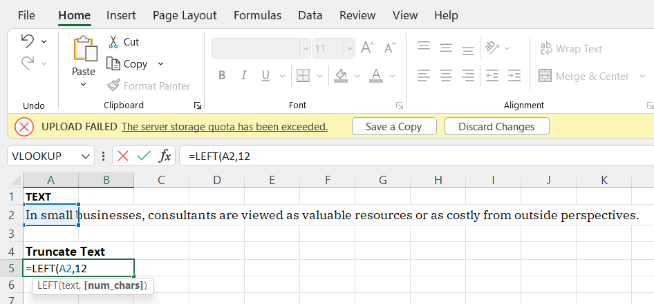
- Enter when the formula is complete.
Read more: How to Insert Multiple Rows in Excel
Method 3. MID
The MID and MIDB functions are used when you want the text you want to maintain to be located in the middle of a string of text. By specifying an appropriate number of characters, the MID FUNCTION removes characters from the middle of the text.
- Choose the cell wherein you would like the truncate text in Excel to be shortened.
- Enter the MID formula in the cell where you want it to appear. i.e: =MID(A2,7,12)
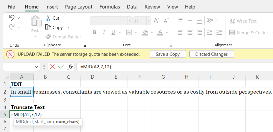
- Now press Enter to submit the formula.
Conclusion
As an alternative to the RIGHT function, we can use the RIGHT function to truncate the text, which displays only the last few characters as stated in the formula. A formula or function will rarely be sufficient to solve the issue at hand. For the most part, you will need to achieve something more complicated. Rather than spending hours on research and aggravating yourself, you might want to consider our strategies.
Leave a Reply