You can make negative numbers red in Google Sheets easily. I have shared three different ways to make any type of – negative number in Red color or even in any other different color.
Negative numbers are those that are less than zero, and Excel automatically prefixes them with a minus symbol. If you use Google Sheets to keep tabs on your finances, you’re bound to come across some negative statistics. To make negative numbers more visible, you can have them show in red automatically, which is considerably more visible than a minus sign or parenthesis.
How to Make Negative Numbers Red in Google Sheets
The three approaches to make negative numbers red in Google sheets are:
- Using Conditional Formatting
- Using Custom Formatting
- Using number Formatting
Assume you have the following dataset.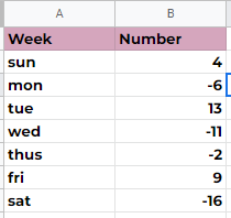
Read more: How to Make a Gantt Chart in Google Sheets
Method 1. Using conditional Formatting
You can format a cell based on its contents using conditional formatting. With conditional formatting, it is possible to change the font color of negative numbers without changing the format.
To make negative numbers red in Google Sheets, follow these simple steps:
- Choose the cell range that you want to use.
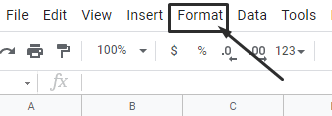
- Select the Format menu option.
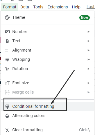
- And choose “Conditional Formatting.”
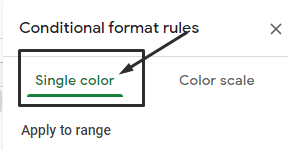
- At the top, click the Single Color tab and verify the cells chosen in the Apply To Range box.
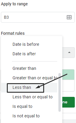
- Select the ”Format cells if” option.

- Select the ”Less than” option from the drop-down menu.
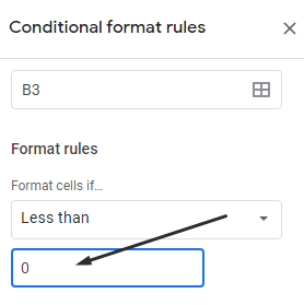
- Input 0 in the ”Value or Formula” section.
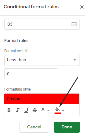
- Now, set the cell’s highlight color.
- Then click on Done.
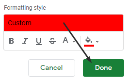
- All cells with a value less than 0 would be immediately displayed by the above steps.
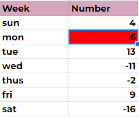
If the cell value changes, the formatting in the cell is instantly updated since conditional formatting is dynamic.
Read more: How to Create a Graph in Google Sheets
Method 2. Using Custom Formatting
Using a custom number format in Google Sheets, you can turn a range of cells red. This will highlight only negative numbers.
- Go to Google Sheets, login in if necessary, and open the spreadsheet that you created.
- Pick the cells which have or may have negative numbers.
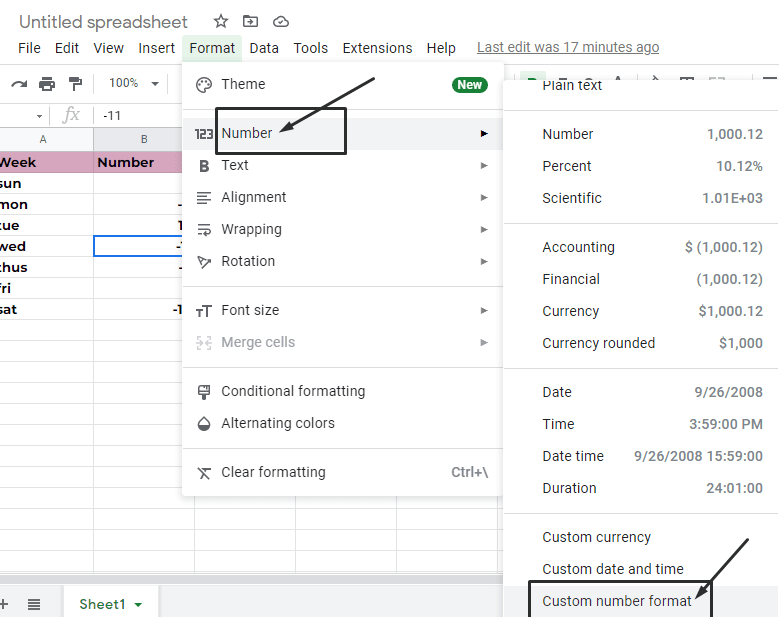
- In the menu, choose the Format tab.

- Now, select “Custom Number Format” from the Number drop-down menu on the Format tab.
- Fill out the next box to choose how you want your numbers formatted: #,##0.00_);[Red](#,##0.00).
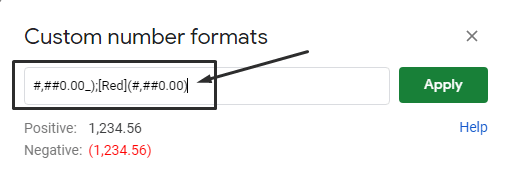
- Select the Apply option.
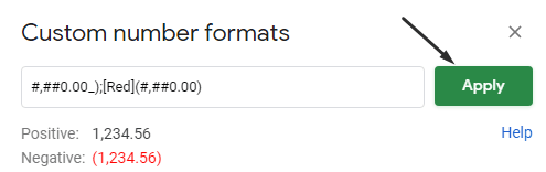
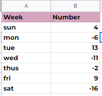
Now, despite everything else in your dataset remaining the same, the negative numbers would be highlighted in red.
Read more: How to Make a Spreadsheet in Google Docs
You can also choose from many number formats if you use custom number formatting:
- Positive numbers
- Negative numbers
- Zero values
- Text values
Read more: How to Group Worksheets in Excel
Method 3. Using Number Formatting
- Select cell range and datasheet.
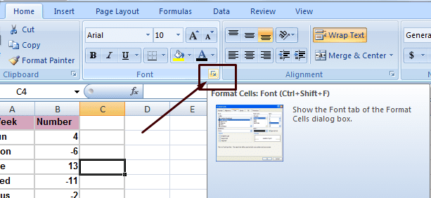
- Go to Excel’s Home tab and select the little arrow-shaped icon to expand the Number group’s numerical formatting.
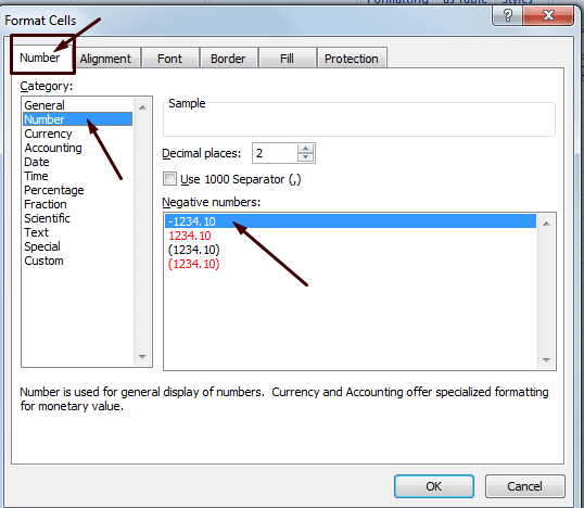
- In this section, you can format cells and change the cell’s formatting to suit your needs. From the drop-down menu on the window’s left side, choose “Number” or “Currency.”Choose negative numbers (1234.10) and press the OK tab.
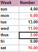
- When you return, you’ll find a red mark on a negative number.
Read more: How to Make a Timeline on Google Docs
Conclusion
Conditional Formatting should be used with caution when displaying negative numbers since it reassesses its condition and applies to format again if the number changes. You can even change the colour of the text using custom formatting. However, Text formatting does not support colours.
A variety of colors are available, including black, red, blue, yellow, and green. So, I’ve listed 3 ways to make cell values with negative values stand out in red. I prefer to format negative numbers using custom formatting instead of using built-in functions in most programs.
Leave a Reply