How to Cross Reference Two Lists in Excel

You can cross reference two lists in Excel by following these five methods. All these methods are easy, and by writing a small command, you can check the reference of two lists. This method work on Excel 2019, 2016 and 2013.

You can choose from many different approaches, and the one that best suits the data structure and the needs of the specific user will be chosen. Suppose, for instance, that you cross reference two lists in excel and want to identify or highlight all the identical data points (that appear in both columns), or just the differences (where a data point appears in one column but not the other), or something along those lines.

Moreover, Excel’s MATCH and IF functions, as well as the ability to highlight rows that differ, make it simple to find similarities between lists. The process of manually finding differences between two lists can be time-consuming and error-prone. Avoid doing so! Since the process will take up a significant amount of time.

Excel allows you to highlight changes in values quickly and easily with the conditional formatting function. Using this metric, you will be able to gauge the number of lines in the columns that differ from one another.

MATCH Method
IF Method
VLookup Algorithm
Duplicate functionality
Conditional functionality

Method 1. MATCH Method

First, let’s review the MATCH function from Excel’s fundamentals so that we may compare two lists to see if they match. Using MATCH, you may find the item’s position in a range. Moreover, The MATCH function allows you to determine whether or not an item from a cell in List1 occurs in List2.

By returning the row position of this item in List2, the function verifies its existence. The #N/A symbol indicates that the text in the cell doesn’t appear in the second list.

After making two lists, Enter MATCH in a blank cell is required.
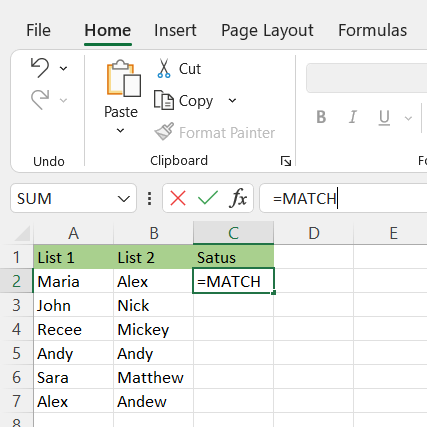
As the first parameter for MATCH, you must specify the Lookup_value.
Make the MATCH function take a second argument that specifies the Lookup_array.
Thirdly, enter the argument to the MATCH function.
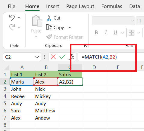
For the remaining cells, drag the lower right corner downwards using the same method.

In List2, you can now see which rows contain the items.

Method 2. IF Method

By comparing two lists with the IF Function in Excel, you can determine if there are any matches in the same column. When the values are the same, a function will return TRUE, and if they are not, FALSE. In other words, if a criterion is met, the display of “Match” appears, whereas if it isn’t, “Not a Match” appears.

The IF function must be entered into an empty cell.
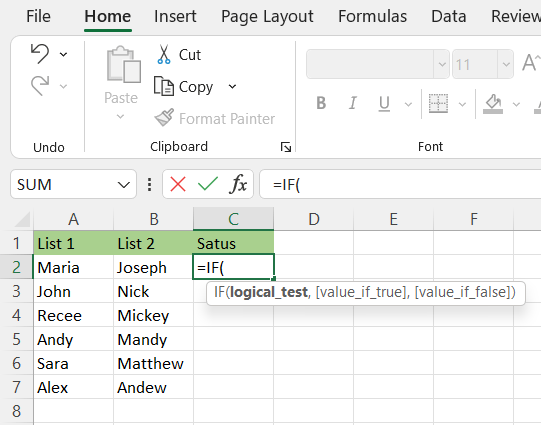
The first parameter for the IF function must be entered.
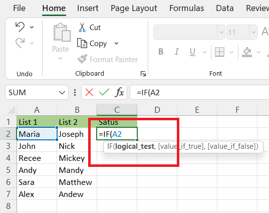
Specify the second argument for the IF function.
As the third argument in the conditional expression IF, specify Value if false.
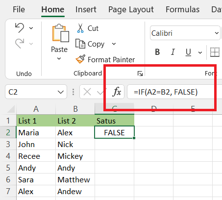
By dragging the lower right corner downwards, the values in the other cells can also be changed.

Method 3. VLookup Algorithm

Here’s an example: I have two Lists, one with a list of names, as shown in the screenshot below. I would like to cross reference two lists in Excel and see which names are the same between them. Comparing two sheets of data manually is tedious, so in this blog post, I’ll demonstrate some shortcuts that will speed up the process.

To get started, open your Microsoft Excel document.
Choose the cell immediately adjacent to the first item on your second list.
Using the empty cell, enter =vlookup(.
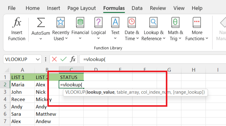
Select the cell or just type A2.
In the formula, include a comma.
To select the first list, hold down the shift key and click on it.
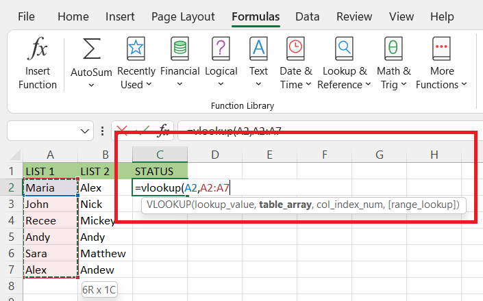
After the comma, enter the number 1 and again put the comma.
In the formula, enter FALSE.
Complete the formula by typing ) at the end.
To submit your entry, press Enter or Return on your keyboard.
Click on the formula cell to choose it after your formula has been executed and the results have been displayed for the first item in the list.
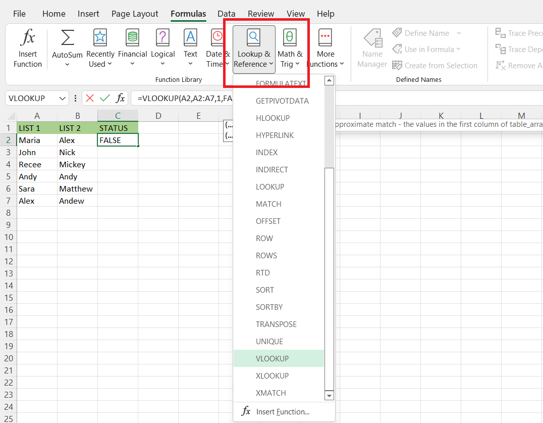
By clicking and dragging the green dot at the bottom right corner of the cell, you can lower it.

Method 4. Duplicate functionality

By using the duplicate functionality in conditional formatting, you can cross reference two lists in Excel. By comparing each row, we can see this is a new result. This situation does not require a row-by-row comparison.

Make a selection of the complete data set.
Navigate to the Home section.
To learn more about the ‘Conditional Formatting’ option in the Styles category, click here.
Click on the Highlight Cell Rules option.
Select Duplicate Values from the drop-down menu.
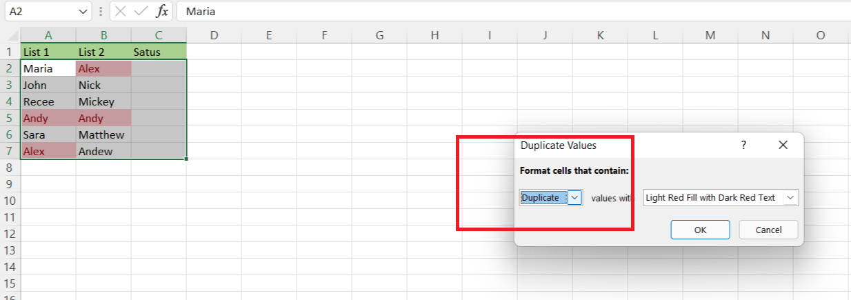
In the Duplicate Values dialogue box, choose ‘Duplicate’. The formatting needs to be specified.
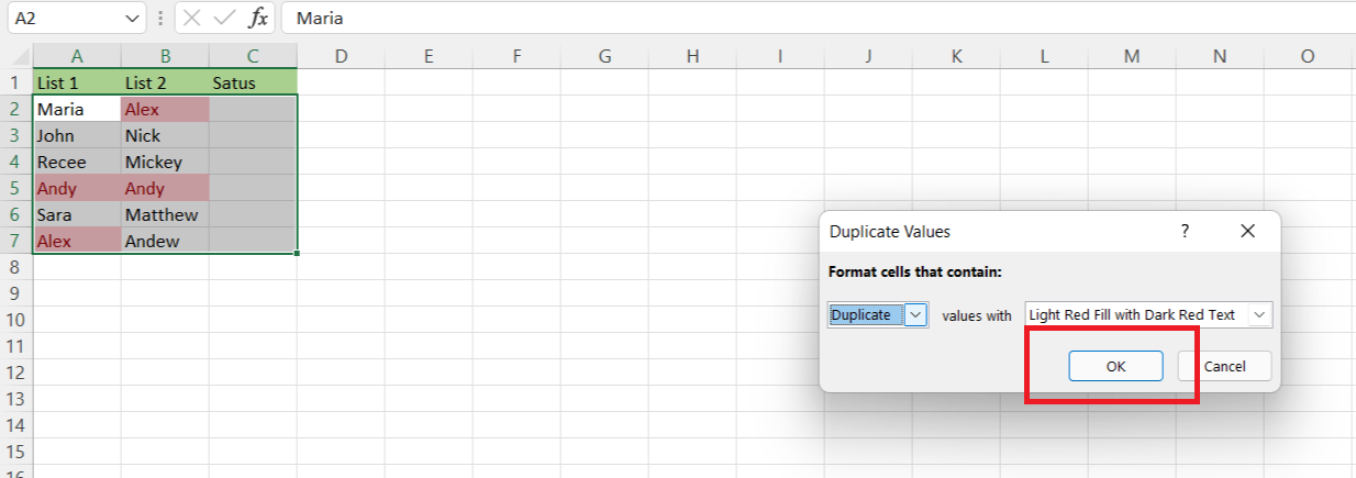
Select OK.

Method 5. Condition functionality

By using Conditional Formatting, you can make sure the rows with the most matching data are highlighted (rather than having the data appear separately in a column).

Select the complete collection of data.
Go to the ‘Home’ option.
Select ‘Conditional Formatting’ from the Styles menu.
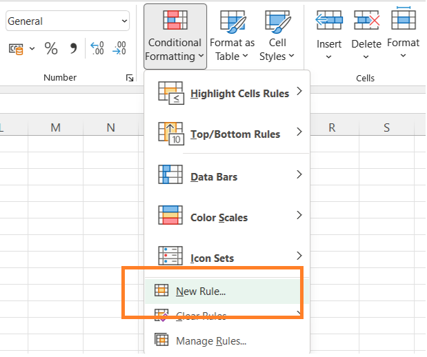
Select ‘New Rule’.
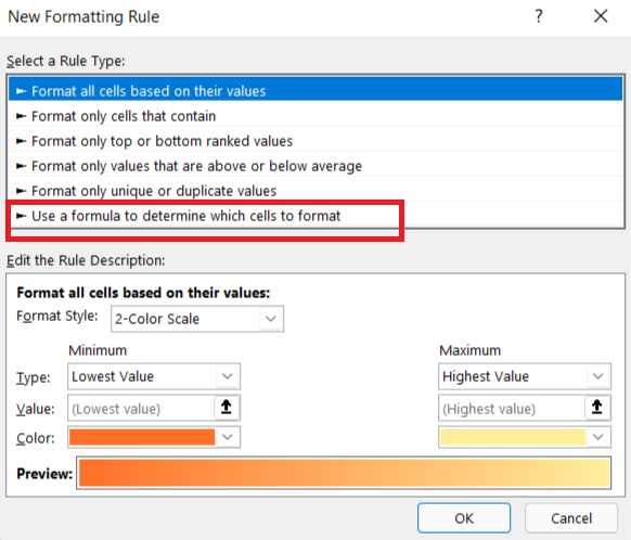
From the ‘New Formatting Rule dialog box, choose ‘Use the formula to select which cells to format’.
Enter =$A2=$B2 in the formula area.
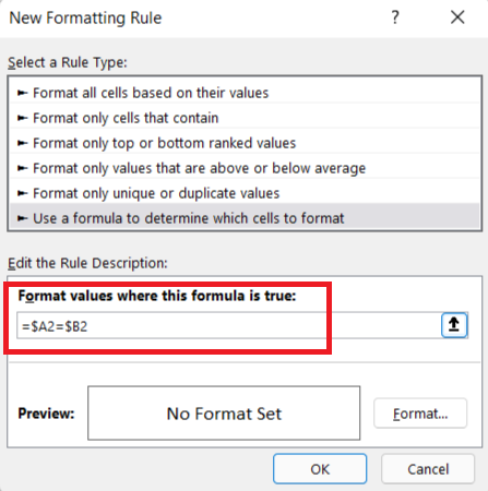
Then, select the Format button and enter the formatting for the matching cells.
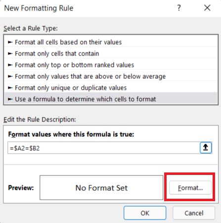
To finish, click the OK button.

Referencing data in another Excel document

Whenever a cell in Excel is linked to another worksheet, the cell that contains the link displays the same information. As the cell in the worksheet to which the link is made. To avoid errors, it is critical that the formula be accurate. To cross reference Two sheets in excel is quite easy.

Make sure both Excel files are open.
To reference a cell in another file, type an equal sign (=), navigate to the other file, and then click and press enter on the cell that you wish to reference in that file.
Determine the name of the workbook, the sheet, and the cell.
In the formula bar of the worksheet, you want to refer to, write the following: [FinancialSample.xlsx] Sheet1!D2.
After clicking enter, you will see the results. It is not a problem that there are multiple ways to access a document.

Conclusion

When you cross reference two lists in Excel, the data structure will have an impact on how these techniques are used. It is not recommended to use a row-by-row matching method when the data is disorganized. Moreover, You can use cross-references to refer to data in another part of the same spreadsheet when you use cross reference two lists in Excel.

Also, you need to understand how to locate cells within multiple workbook sheets using their extended address format in order to cross-reference between sheets.

Was this article helpful?

YesNo

How to Cross Reference Two Lists in Excel – Top 5 Methods