You can create slicers in Excel by following these methods. You can create a slicer of numbers or any format in an appealing way. These methods will work in 2013, 2016, and 2019.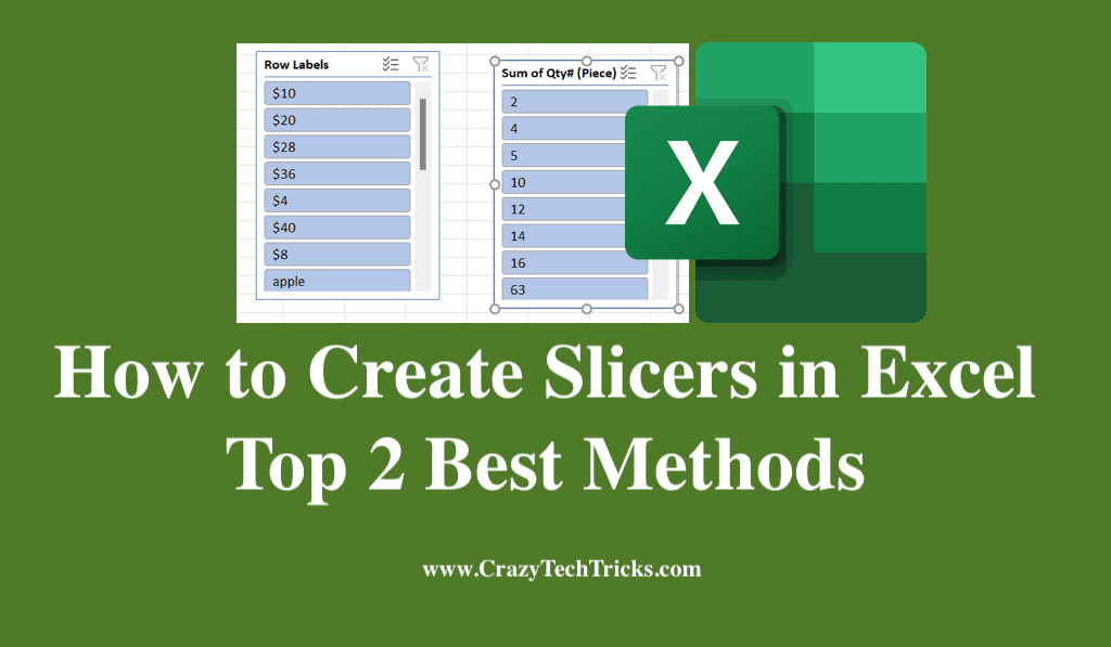
Essentially, a slicer is an on-screen tool for filtering data in a spreadsheet’s table rows and columns. You can filter tables or PivotTables using Slicer keys. Moreover, slicers show the current state of the filtering, making it easy to see what is currently being presented.
Read more: How to Increase Size of Taskbar in Windows 11
For example, suppose you have a data table containing information about different countries. In that case, you can create a slicer that will only display records whose country is the United States of America (USA). Slicers, however, allow you to filter data while keeping track of what’s being filtered in your Excel. So, in this article, we’ll show you how to create slicers in Excel.
Read more: How To Combine Two Columns in Excel
How to Create Slicers in Excel
There are two ways to create slicers in Excel. These are
- Insert Tab
- PivotTable Analyze tab
Read more: How To Combine Two Columns in Excel
Method 1. Insert Tab
To process to create Slicers in Excel using Insert tab are as follows:
- To begin the process of creating a slicer, open your excel in Excel.
- After that, select the table in which you wish to apply a slicer to filter content.
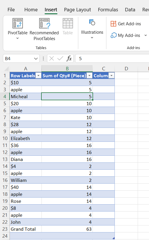
- Choose your table and then click the “Insert” option in the top-right corner of Excel’s ribbon.
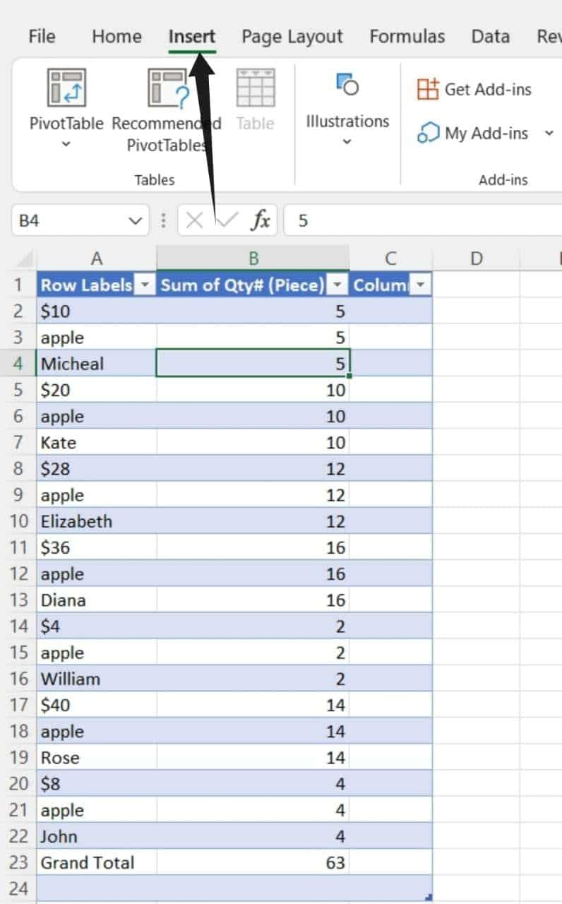
- Now, To add a slicer, click the “Slicer” button under the “Filters” section on the “Insert” tab.
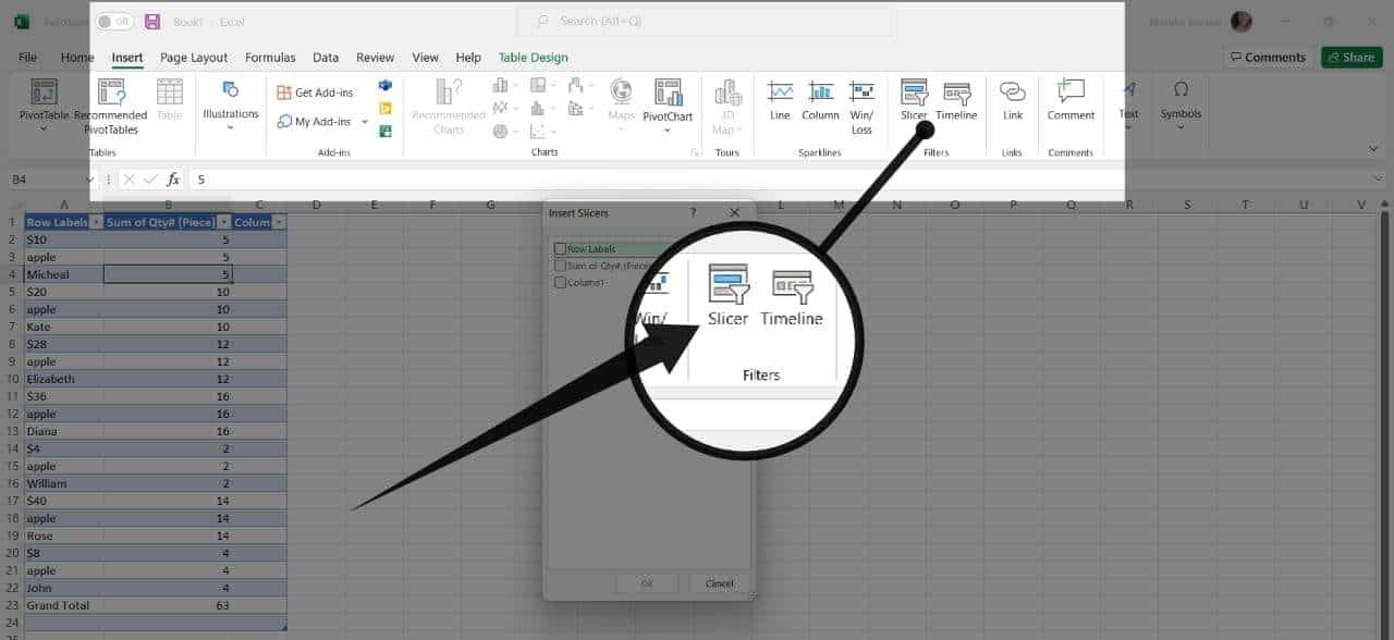
- The variables of your table will be displayed in the “Insert Slicers” dialogue.
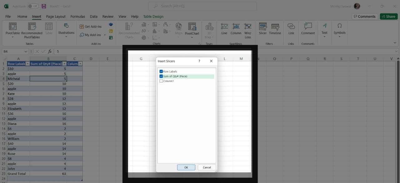
- Then, at the bottom of the page, select the fields that you wish to filter using a slicer and click “OK.”
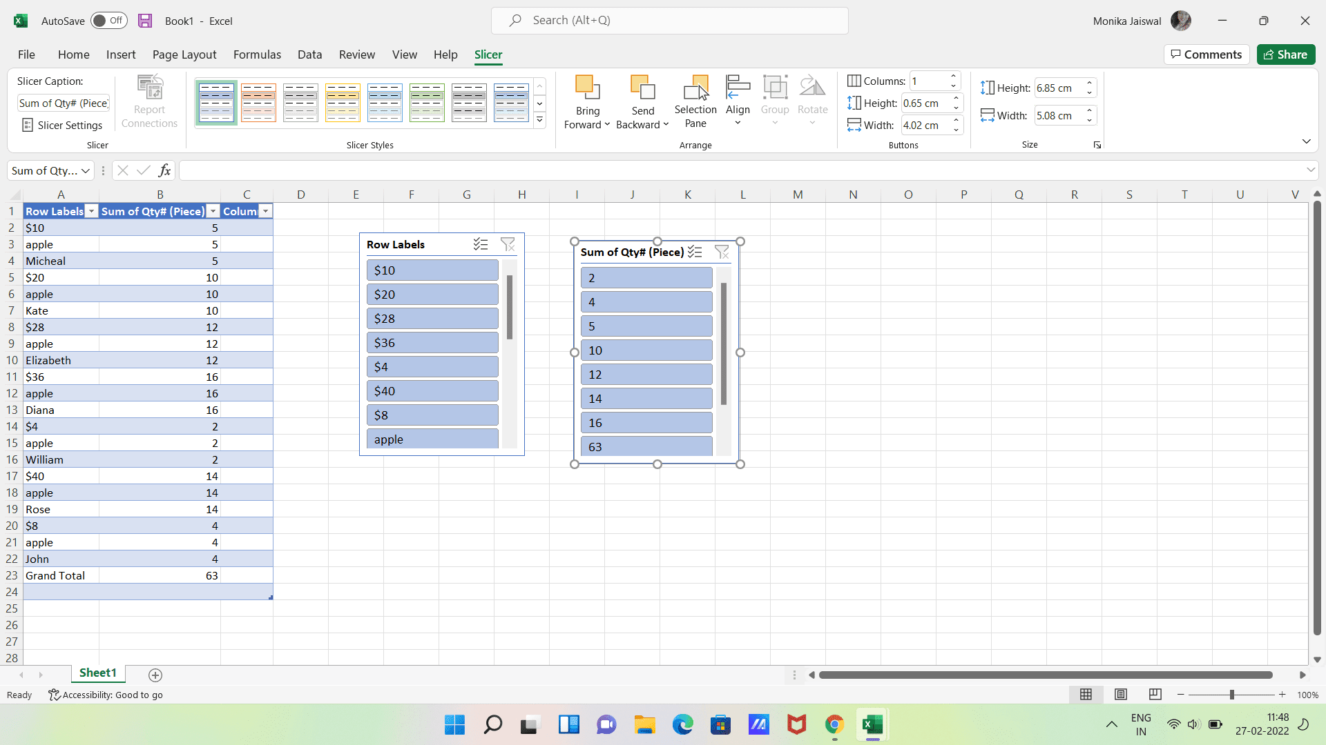
- For each field you choose, Excel will add a slicer. By selecting an option within one of these slicers, you can begin filtering your data.
Read more: How to Add a Secondary Axis in Excel
Method 2. PivotTable Analyze Tab
Alternatively, you can view the same list of fields under the PivotTable Analyze tab. Well, I’ll guide you through how to use the PivotTable analysis tab to create slicers in Excel.
- Select a cell in the pivot table by clicking on it.
- To insert a slicer in Excel 2013, Excel 2016 and Excel 2019, go to Analyze > Filter > Insert Slicer.
- Now, Insert slicers pop up will appear. More than one slicer can be added here simply by selecting more than one cell.
- Click OK once done.
Read more: How to Insert Multiple Rows in Excel
Customize the look of the slicer in Excel
Are you searching for something more than Excel’s built-in slicer styles? You can create your own! Here’s a step-by-step guide.
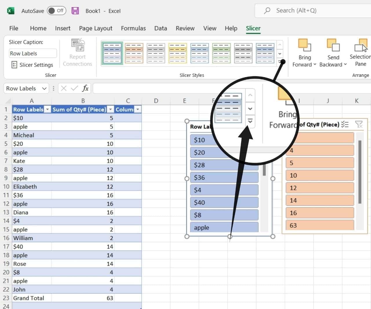
- In Slicer Tools Options, click on More under the Slicer Styles group.
- To add a new Slicer Style, click on the Add New Slicer Style button at the bottom of the gallery.
- Assign the name according to your wish on your new style.
- Select a slicer element, click the Format button, and customize the element’s formatting choices.
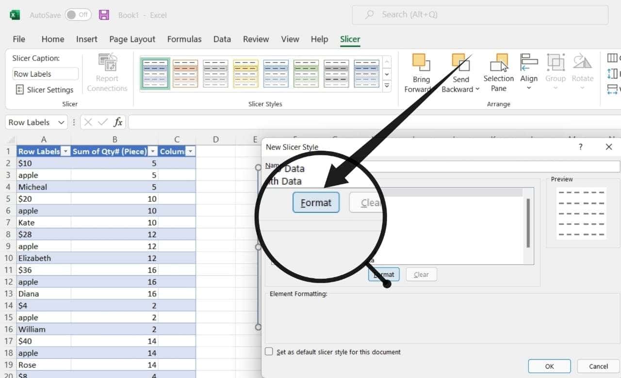
- Then go on to the next part of your plan. When you click OK, your new style will be added to the Slicer Styles Gallery.
Note:
With Excel 2010, you can only use a slicer to work with pivot tables. Whereas, In Excel 2013 and later, you can add a slicer to either pivot tables or conventional tables, depending on your preferences.
Read more: How to Use Exponents in Excel
Conclusion
The Insert Slicers window is beneficial because several slicers can be simultaneously inserted into various fields. Using slicers, your Excel reports will have a professional appearance. They’ll also give a wonderful level of interactivity to your otherwise static panels. In most cases, adding Slicers to a pivot table is straightforward. However, if the pivot table was created in an older version of Excel, you may need to upgrade. Finally, I’d like to conclude my blog post here by conveying my hope that you found this article to be helpful.
Leave a Reply